I’ve been curious about machine learning for a while but I never found a project that I was interested enough in to make me overcome my fears of not being able to do anything, being a complete beginner. I was introduced to this competition a couple of days after Kaggle opened it up and I became very interested after learning the implications of this project. To give a brief background, the Grasp and Lift EEG Kaggle competition aims to create a BCI machine that will help patients needing prosthetics arms move their arms with their brain activity as they would normally. Twelve subjects were recorded moving their arms and grasping-and-lifting and object. The EEG data contains 32 channels and around ~20 trials in each series, recorded at a sampling rate of 500 Hz. Another file is attached for every series containing the exact labels for when each of the 6 events (classes: HandStart, FirstDigitTouch, BothStartLoadPhase, LiftOff, Replace, BothReleased) which we are supposed to predict correctly.
I’ve gotta thank Kaggle’s script and forum sections of this competition as these really helped me get started and understand this whole new field to me. In this post I’ll be describing what I’ve learned, what I’m currently learning/working on and what I want to do in the future with this competition. When I started, I began exploring the data by uploading the data as python pandas data frame. Since the data was recorded at a sampling rate of 500 Hz, this means that a reading from each channel electrode was taken every 0.02 seconds (sampling rate = 1/t => t = 1/sampling rate). As a result, every file has a substantial amount of rows of samples, making the data set very large, sample wise. The 32 raw channels serve as our feature vectors, but the channels themselves aren’t very informative. Running logistic regression on the raw data itself (just scaling the train and test data about zero before running the machine learning algorithm) returns a score of ~70% accuracy of classifying each class. Another thing about the data is that the EEG readings are really noisy and the frequency bands of interest, alpha and beta, are in a very small frequency range compared to the range of frequencies found in just one channel of the EEG data. For BCI based on oscillatory activity (i.e. motor imagery-based BCIs such as moving an arm), the frequency bands of interest are alpha (7-12 Hz) and beta bands (12-30 Hz). Conforming to Nyquist criterion: sampling at twice the highest frequency content of the signal, implies that the signal’s highest frequency component is around ~250 Hz, which leaves a lot of room for noise we won’t need to detect the hand movement). For motor imagery-based BCIs, we need to use spectral and spatial information to get better and more informative feature vectors.
After discovering this information, I first tried to experiment with the machine learning algorithm I wanted to use. At first, after some research, I decided to try out a Support Vector Classifier as we are supposed to classify the signals into six labels. However, for this competition, it was preferred that we submit a file with the probability of each trial belonging to a certain class instead of a definitive binary 0 or 1 for each class. Sklearn’s SVM library does provide a predict_proba() function to provide the probability for each class but it is not very accurate. The accuracy score was closer to ~50%, lower than using simple logistic regression whilst doing nothing to preprocess the data.
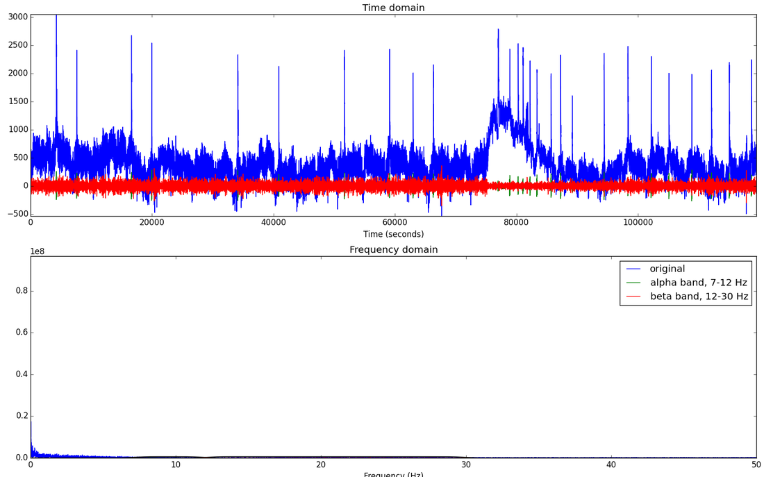
Clearly experimenting with the choice of model was not very fruitful at this point and it was more likely that I could get a higher accuracy if I did some feature engineering with the raw data I was already using. Doing some more reading and research on how people handle EEG data, I began looking into basic signal processing. The following is the more recent things I’ve done. As mentioned earlier, the best frequency bands to use for classifying movement are alpha and beta bands which are in the 7-30 Hz range. One idea is to try to isolate these alpha and beta frequencies and use their power spectrum to see just where and when a hand/arm movement is occurring. Since we are interested in certain frequency ranges, I decided to do FFT on each individual channel and visualize the different frequency bands. This really helped see just how noisy the signals where and see how strong these frequency bands of interest are. Here is a plot of the first channel, just filtering for the alpha and beta frequency bands.
I’ve gotta thank Kaggle’s script and forum sections of this competition as these really helped me get started and understand this whole new field to me. In this post I’ll be describing what I’ve learned, what I’m currently learning/working on and what I want to do in the future with this competition. When I started, I began exploring the data by uploading the data as python pandas data frame. Since the data was recorded at a sampling rate of 500 Hz, this means that a reading from each channel electrode was taken every 0.02 seconds (sampling rate = 1/t => t = 1/sampling rate). As a result, every file has a substantial amount of rows of samples, making the data set very large, sample wise. The 32 raw channels serve as our feature vectors, but the channels themselves aren’t very informative. Running logistic regression on the raw data itself (just scaling the train and test data about zero before running the machine learning algorithm) returns a score of ~70% accuracy of classifying each class. Another thing about the data is that the EEG readings are really noisy and the frequency bands of interest, alpha and beta, are in a very small frequency range compared to the range of frequencies found in just one channel of the EEG data. For BCI based on oscillatory activity (i.e. motor imagery-based BCIs such as moving an arm), the frequency bands of interest are alpha (7-12 Hz) and beta bands (12-30 Hz). Conforming to Nyquist criterion: sampling at twice the highest frequency content of the signal, implies that the signal’s highest frequency component is around ~250 Hz, which leaves a lot of room for noise we won’t need to detect the hand movement). For motor imagery-based BCIs, we need to use spectral and spatial information to get better and more informative feature vectors.
After discovering this information, I first tried to experiment with the machine learning algorithm I wanted to use. At first, after some research, I decided to try out a Support Vector Classifier as we are supposed to classify the signals into six labels. However, for this competition, it was preferred that we submit a file with the probability of each trial belonging to a certain class instead of a definitive binary 0 or 1 for each class. Sklearn’s SVM library does provide a predict_proba() function to provide the probability for each class but it is not very accurate. The accuracy score was closer to ~50%, lower than using simple logistic regression whilst doing nothing to preprocess the data.
Clearly experimenting with the choice of model was not very fruitful at this point and it was more likely that I could get a higher accuracy if I did some feature engineering with the raw data I was already using. Doing some more reading and research on how people handle EEG data, I began looking into basic signal processing. The following is the more recent things I’ve done. As mentioned earlier, the best frequency bands to use for classifying movement are alpha and beta bands which are in the 7-30 Hz range. One idea is to try to isolate these alpha and beta frequencies and use their power spectrum to see just where and when a hand/arm movement is occurring. Since we are interested in certain frequency ranges, I decided to do FFT on each individual channel and visualize the different frequency bands. This really helped see just how noisy the signals where and see how strong these frequency bands of interest are. Here is a plot of the first channel, just filtering for the alpha and beta frequency bands.
After visualizing it, I thought that filtering each channel with FFT would be a good way to go. After trying to filter the data with FFT, the results were not very promising. Going back to the drawing board and doing some more reading on the nature of EEG signal processing,
I wanted to obtain these specific band ranges in a fast and simple way, and after some digging, I found that using a bandpass filter of some kind would be a good way to go. A bandpass filter only filters for frequencies in a certain frequency band, which is exactly what I was looking for. One specific type of filter that I saw that was used frequently in this competition is the Butterworth filter. After obtaining the different frequency bands of interest from the data, I took those frequency bands and took their power spectrum as added feature vectors. The power of a signal is proportional to the magnitude squared, i.e
Power(signal) = (frequency band magnitude)^2.
So the final feature vectors that would be fed into the model include the raw data, the specific frequency bands of interest, and their power spectrum. This resulted in a total of 52 feature vectors, an increase from the raw data 32 feature vectors. Using spectral information greatly helped improve the performance of the model, now at 80% accuracy, an increase of 10%. Another useful source of information is using spatial information. Spatial information focuses on determining where (which channels) does the relevant signal come from. A very common algorithm used in EEG data to extract spatial information is the Common Spatial Pattern (CSP) algorithm. Unfortunately, python’s sklearn library doesn’t have an easy built in function to run, and I’ve looked at other libraries that have this algorithm but I still haven’t gotten the hang of how to get these to work. I’m working on writing my own implementation of this algorithm (still learning the technicalities of how it’ll work with my data).
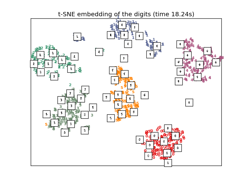
Here's also a little T-SNE demo I did to learn about it using MSNE data (images of numbers of which we are trying to classify in their respective clusters)
In the very near future, I want to try to use T-SNE on the data (including the spectral and spatial information feature vectors) to further discriminate when a certain signal at some point in time belongs to one of the 6 events that we are trying to classify. T-SNE is primarily an algorithm that helps with the visualization of clusters within the data. The algorithm takes a high dimensional data space [R^d d = 52+ in this case] and reduces its dimensionality down to 2 or 3 dimensions. It uses the euclidian distance between the points in the R^d space and tries to replicate the same kind of euclidean distance between the points that have been projected onto the new 2D space to visualize the nature of the data in a reduced dimension. Then it defines a conditional similarity between the mapped points and can define a similarity matrix for the mapped points to cluster similar signals (points) together into the 6 events (classes). After having the data processed this way, I believe using KNN (K Nearest Neighbors) will make classification extremely effective. KNN is an algorithm that does not generate a function to divide the data like SVM and logistic regression do. Instead, KNN measures the distance between the points around it (neighbors) and a specific amount of points (determined number of neighbors)with the shortest distance around a point will be set as a cluster for a class. The algorithm will go through all the data and draw boundary lines between all the different clusters found. When a new point is introduced (test data point), it’ll calculate its euclidean distance once again to the points around it and classify it to one of the clusters found earlier. I think this approach will make the score jump at least a little higher since we are classifying for more than two classes. The other two models I previously used are binary in the sense that there is only one division (a function line or function of some sort) to divide the data. Perhaps aiming to classify the signals into every event will allow for increase in accuracy. I have yet to see if this is true, but will do soon enough.

 RSS Feed
