This spring semester, I am taking a class in signal processing and I am very excited to learn more about Fourier Analysis. For the Kaggle EEG contest I wrote about months ago, there were many signal processing techniques I was reading about but I didn't get to fully dive into the theory behind some of these tools. I think I'll be writing a series on new things I learn from this class and try to show some tutorials in coding and applying some of these techniques.
Fourier Series
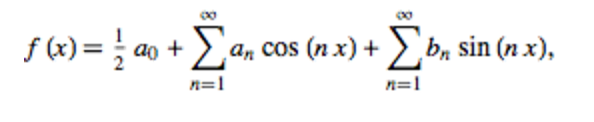
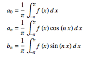
Our introduction to Fourier Analysis begins with learning about Fourier Series. Basically, if you have a function that is 1. p-periodic and 2. Riemann integrable on every bounded interval, then you can approximate (decompose) that function into a sum of trigonometric polynomials-- a sum of sines and cosines each with a weight a_n, b_n determined by the following formulas:
Fourier Series
Our introduction to Fourier Analysis begins with learning about Fourier Series. Basically, if you have a function that is 1. p-periodic and 2. Riemann integrable on every bounded interval, then you can approximate (decompose) that function into a sum of trigonometric polynomials-- a sum of sines and cosines each with a weight a_n, b_n determined by the following formulas:
|
|
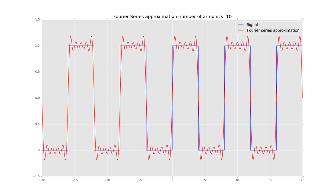
For example, we can use a Fourier Series to decompose the square wave function with period = 8. Here we are using a Fourier Series that sums up to N = 10.
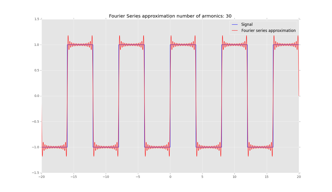
The bigger we make the sum, the better the approximation becomes. For example here is that same Fourier series with the sum being up to N = 30.
Fourier Transform
The Fourier transform takes the Fourier series you used to approximate your function and spits out the frequencies and amplitudes of the series to describe the basic components of your function. In other words, a Fourier Transform tastes a dish and spits out the recipe.
The Fourier transform takes the Fourier series you used to approximate your function and spits out the frequencies and amplitudes of the series to describe the basic components of your function. In other words, a Fourier Transform tastes a dish and spits out the recipe.
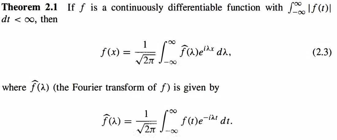
This theorem is known as the Fourier Inversion formula, which states that f(x) can be described in terms of its Fourier Transform. This technique can be used to tag songs based on their frequency signatures, allow you to compress files, and used in image processing.
I followed a tutorial from OpenCV that shows how to use OpenCv and numpy in python to do some basic image processing. Here is what I got from the tutorial:
This code is the numpy version to perform a basic Fourier transform. We first import the image we will be analyzing and immediately perform a Fourier transform on the image. Then after some input/output image adjustments if necessary, we can compute the magnitude spectrum of the image and post them side by side.
import cv2
import numpy as np
from matplotlib import pyplot as plt

img = cv2.imread('PATH TO IMAGE',0)
f = np.fft.fft2(img)
fshift = np.fft.fftshift(f)
magnitude_spectrum = 20*np.log(np.abs(fshift))

plt.subplot(121),plt.imshow(img, cmap = 'gray')
plt.title('Input Image'), plt.xticks([]), plt.yticks([])
plt.subplot(122),plt.imshow(magnitude_spectrum, cmap = 'gray')
plt.title('Magnitude Spectrum'), plt.xticks([]), plt.yticks([])
plt.show()
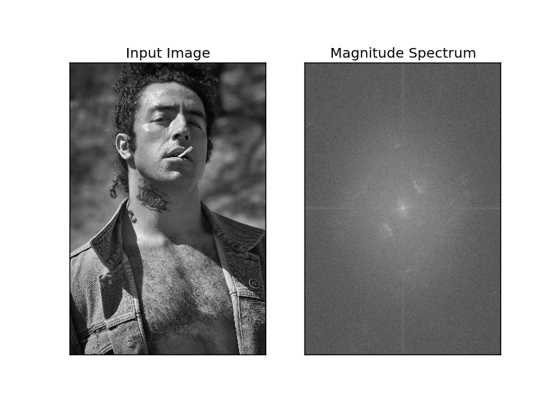
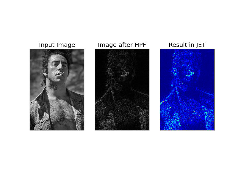
The white spots in the center represent a high concentration of lower frequencies. Boundary lines in images have high frequencies so we can take advantage of this behavior to reconstruct the edges of the image and create almost an "outline" of the input image. We will design a filter that only allows high frequencies to pass through to reconstruct the image later with only these high frequencies. This is called High Pass filtering and it is often used for edge detection. Here we will use the Fourier Inverse theorem that says we can get our original function from the Fourier transform (only this time the Fourier transform will have a High Pass filter applied to it first).
rows, cols = img.shape
crow,ccol = rows/2 , cols/2
fshift[crow-30:crow+30, ccol-30:ccol+30] = 0
f_ishift = np.fft.ifftshift(fshift)
img_back = np.fft.ifft2(f_ishift)
img_back = np.abs(img_back)

plt.subplot(131),plt.imshow(img, cmap = 'gray')
plt.title('Input Image'), plt.xticks([]), plt.yticks([])
plt.subplot(132),plt.imshow(img_back, cmap = 'gray')
plt.title('Image after HPF'), plt.xticks([]), plt.yticks([])
plt.subplot(133),plt.imshow(img_back)
plt.title('Result in JET'), plt.xticks([]), plt.yticks([])

plt.show()
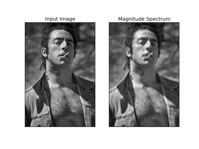
We can do the opposite and filter the Fourier transform to only allow low frequencies to pass through. As you may have guessed this is called Low Pass filtering. The Low Pass filtering will actually blur the image. The code below uses OpenCv instead of numpy.
rows, cols = img.shape
crow,ccol = rows/2 , cols/2

# create a mask first, center square is 1, remaining all zeros
mask = np.zeros((rows,cols,2),np.uint8)
mask[crow-30:crow+30, ccol-30:ccol+30] = 1

# apply mask and inverse DFT
fshift = dft_shift*mask
f_ishift = np.fft.ifftshift(fshift)
img_back = cv2.idft(f_ishift)
img_back = cv2.magnitude(img_back[:,:,0],img_back[:,:,1])

plt.subplot(121),plt.imshow(img, cmap = 'gray')
plt.title('Input Image'), plt.xticks([]), plt.yticks([])
plt.subplot(122),plt.imshow(img_back, cmap = 'gray')
plt.title('Magnitude Spectrum'), plt.xticks([]), plt.yticks([])
plt.show()
Some very neat image processing to start applying some of those theories I've been learning. I'll add some more posts about other more advanced concepts once I finish reading ahead. Here is the OpenCV tutorial I followed and here is the Fourier Series tutorial I followed to create the graphs.


 RSS Feed
