An aspect of intelligence that we wish to emulate is goal-based problem solving. This means that we have an end goal in mind and wish to execute it by making a plan. This is the essence of a search problem: we wish to make a plan, find a path, to execute our goal-- make us reach a goal state. Let's try to visualize this with an example:
Say I have an agent (a robot) that needs to find her way from one city to another. Say I am trying to get from Northridge to Santa Monica Beach in Los Angeles. There are many ways (paths) for the agent to get from Northridge, our starting state, to Santa Monica, our goal state. Say there are are different cities we can stop by to get to our goal state.
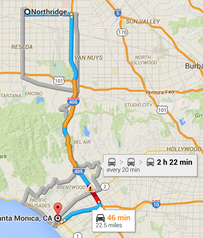
We can draw a map of all the cities between Northridge and Santa Monica and draw different paths we could take. Every city we can cross, including Northridge and Santa Monica will be considered as a node. Here I have a picture of google maps suggesting a couple of routes.
Say I have an agent (a robot) that needs to find her way from one city to another. Say I am trying to get from Northridge to Santa Monica Beach in Los Angeles. There are many ways (paths) for the agent to get from Northridge, our starting state, to Santa Monica, our goal state. Say there are are different cities we can stop by to get to our goal state.
We can draw a map of all the cities between Northridge and Santa Monica and draw different paths we could take. Every city we can cross, including Northridge and Santa Monica will be considered as a node. Here I have a picture of google maps suggesting a couple of routes.
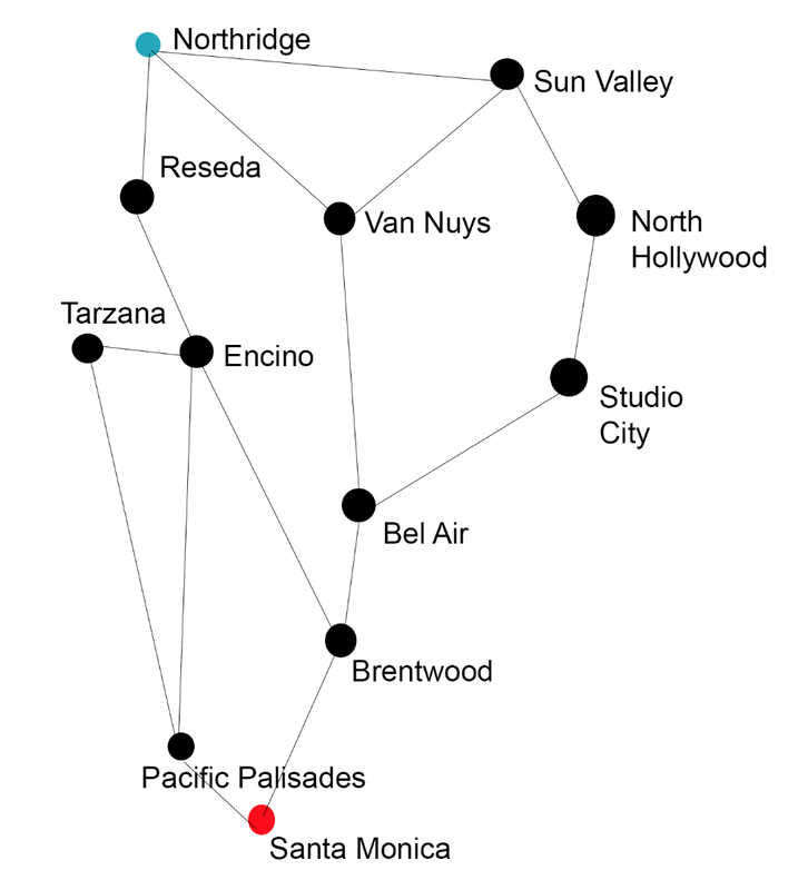
We could make Reseda, Van Nuys, Encino, Tarzana, Bel Air, Brentwood, Pacific Palisades, Studio City, North Hollywood, Sun Valley all nodes. The roads connecting one city to another will be arcs. Then we can translate this map into a graph and view all of possibilities. I've ignored the complicated roads and for the sake of simplicity, let's assume all of the arcs on this graph are roads that the robot can travel on.
Now we have a way to visualize our start and goal states and the different paths that are possible! We can now treat this endeavor as a Search Problem. A search problem consists of:
1. A state space: encodes how the world is at a certain point in a plan; an abstraction of the world.
2. Successor Function: a function that models how you think the world works. It takes the state space and tells you what you can achieve immediately and how much it costs.
3. Start and Goal States: where you begin and where you end
A solution is a sequence of actions which transforms the start state to the goal state. A state space keeps only the details needed for planning.
Sometimes creating the entire search graph for a problem is too big. In this case, the graph isn't that big, but there will be problems where it just would not make sense to attempt to draw the entire graph for the problem. A solution to this would be to draw a Search Tree. A search tree includes the start state (root node--here in blue), goal state (goal node) and children which are successors. The nodes in the search tree correspond to plans that can achieve states. So nodes are plans, not states! When searching with a search tree, we expand out potential plans and maintain a fringe which is a collection of potential plans under consideration. With a tree, we also do not want to expand the entire tree because the tree could also be infinitely large, so we try to keep the expanded amount of notes to be less than the nodes in the tree. Here is an example of what the tree would look like for our search graph above:
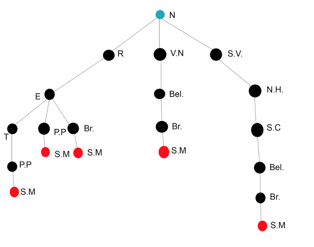
What I've done is basically taken every node and to it attach the nodes that it leads to (making them the child nodes of that one node). For example the children of our starting point Northridge are Reseda, Van Nuys, and Sun Valley.
Now that we have these tools we can begin to discuss different search algorithms to help us get to our goal state. In this post I will discuss two types of search algorithms and I'll leave the rest for another post. The first algorithm we can try is called Depth-First Search, or DFS for short.
Depth-First Search
Depth first search takes a strategy, for example try to expand all nodes to the left first, and tries to get to the bottom of that branch and see if it leads to the goal state. If it does not, then we move on to the next node according to our strategy and do the same thing. What path will this algorithm give us on this problem? Let's work through it. Say our strategy is trying to stick to the leftmost nodes when possible. So we start with our root node Northridge, and place it on our fringe. Whenever we expand a node, we cross it off our fringe, meaning we don't need to expand that node again.
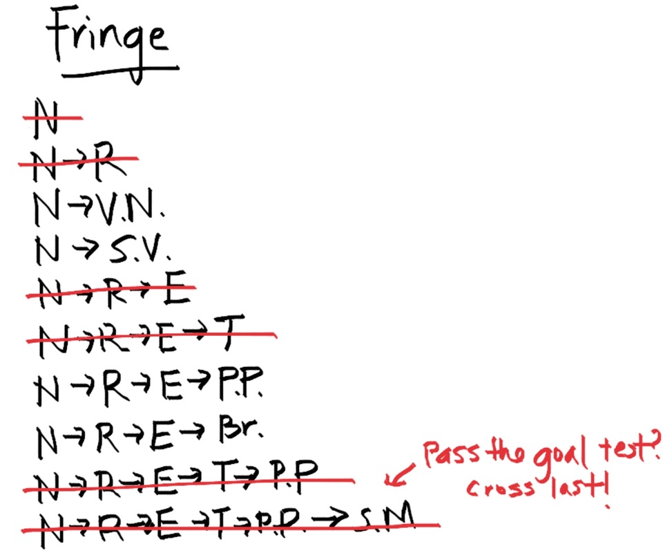

Note we only cross off the last path if it passes the goal test. We check first and if it passes, we take if off the fringe and we're done! So using this algorithm, we see that the path we get is to travel from Northridge, to Reseda, to Encino, to Tarzana, to Pacific Palisades, and eventually get to Santa Monica.
Some properties of this algorithm:
1. It is possible that the only way to get to the goal state would be the very last node it expands, so in theory it is possible that we expand the entire tree! Which is something we really don't want to do if possible. Let b equal the amount of nodes at each level and m equal the depth of the tree (number of levels of the tree). The number of nodes in the entire tree would be 1+b^2+b^3+b^4+...+b^m which we can round to b^m. The state space then would be O(b^m). The fringe only keeps siblings on the path from the root, so the size of the fringe is O(bm). If m is infinite, then this method is not complete (meaning it does not always find the goal). It is definitely not optimal because if we take a look at the tree drawn, there are other paths that are shorter that we could have chosen, but due to the nature of this algorithm we got a suboptimal path.
Breadth-First Search
Breath first search is another search algorithm similar to depth first search. It also has a fringe and we also use a search tree to visualize, but instead of focusing on exploring the entire path on a node till its end, this algorithm focuses on exploring node level by node level first. For example, in this above example looking at the search tree, the BFS algorithm would explore the first tier, N, find that that node itself does not pass the goal test and moves on to the second tier, containing R, V.N, and S.V. Let's keep the same strategy as the other example and try to stay to the leftmost node. At the second tier, the algorithm finds that this layer still does not pass the goal test so it continues down, checking every node in each tier to see if the goal test passes at some node. Here is what the fringe would look like:
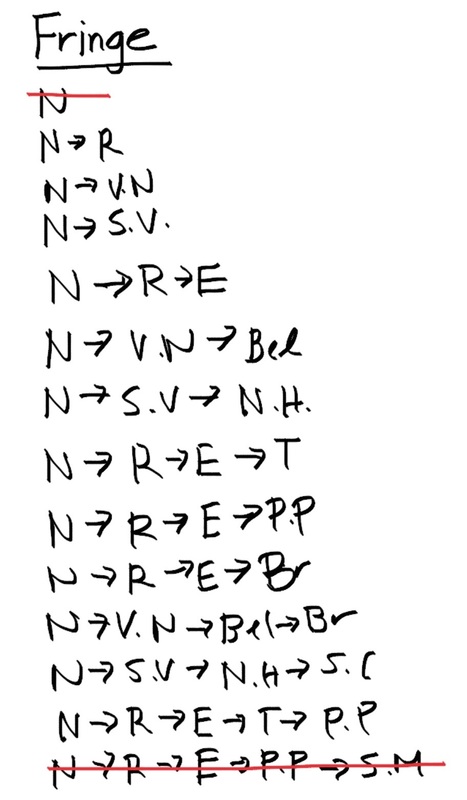
Notice that there are less paths crossed off the fringe. In fact the only path we crossed off was the last one that passed the goal test. Now you can see that the algorithm explores layer by layer to find the shallowest goal node and choose that path. Let s be the number of tiers in which the shallowest goal node resides in a tree. The search space will be O(b^s) because it is guaranteed to stop at the shallowest goal node. The fringe takes the same amount of space O(b^s) because we didn't cross anything off except the last path that passed the goal test. It is complete because s must be finite, so it will always reach the goal state. In general this algorithm is not optimal but if the cost of every arc is equal to 1, then it is optimal.

 RSS Feed
